Voolstra CR, Buitrago-López C, Perna G, Cárdenas A, Hume BCC, Rädecker N, et al. Standardized short-term acute heat stress assays resolve historical differences in coral thermotolerance across microhabitat reef sites. Glob Chang Biol. 2020;26: 4328–4343. doi:10.1111/gcb.15148
Voolstra CR, Valenzuela JJ, Turkarslan S, Cárdenas A, Hume BCC, Perna G, et al. Contrasting heat stress response patterns of coral holobionts across the Red Sea suggest distinct mechanisms of thermal tolerance. Mol Ecol. 2021;30: 4466–4480. doi:10.1111/mec.16064
Upload your datafiles and run Coracle
UniCorP applies UniCor in a bottom-up propagation across the hierarchy. At each level it evaluates features within their parent group, selects UNICORNs using a top-k rule (k highest scores per level) and propagates selected features to the next higher level (e.g., species → genus). This repeats until the highest level is reached, enriching upper levels with informative features.
Scoring can use Pearson or Spearman correlation. An optional preprocessing step for scoring can apply relative abundance or CLR to reflect compositional structure. These settings affect scoring only; propagation is determined by the selection rule at each level.
The selection rule influences group sizes across levels. With top-k per level, the number of propagated features is fixed by k, which stabilizes group sizes and runtime across levels. Overall, runtime grows linearly with the number of samples and with the number of hierarchical levels processed.
Upload your datafiles and run UniCorP
Bottom-up (UniCorP): Starting at the lowest (most specific) hierarchical level, UniCorP identifies uniquely correlated features (UNICORNs) within each group and propagates only the selected features upward. This repeats level by level until the highest (least specific) level is enriched.
Top-down skimming (TDS): From the enriched highest level, UniCoracle selects informative groups and propagates them downward through the hierarchy. This reduces the number of features that reach the lowest level.
Modeling: At the lowest level, the reduced feature set is analyzed with Coracle to quantify associations between features and the continuous target variable.
Voolstra CR, Buitrago-López C, Perna G, Cárdenas A, Hume BCC, Rädecker N, et al. Standardized short-term acute heat stress assays resolve historical differences in coral thermotolerance across microhabitat reef sites. Glob Chang Biol. 2020;26: 4328–4343. doi:10.1111/gcb.15148
Voolstra CR, Valenzuela JJ, Turkarslan S, Cárdenas A, Hume BCC, Perna G, et al. Contrasting heat stress response patterns of coral holobionts across the Red Sea suggest distinct mechanisms of thermal tolerance. Mol Ecol. 2021;30: 4466–4480. doi:10.1111/mec.16064
Runtime complexity. UniCoracle is less sensitive to very large feature sets than Coracle because it first restricts computations to within-group correlations during bottom-up propagation and then limits the number of features passed downward during top-down skimming.
Bottom-up (UniCorP): The dominant cost per level is computing correlations within groups, which scales as with n samples and features in group g. Using top-k selection per level keeps the number of propagated features fixed and stabilizes runtime.
Top-down skimming (TDS): Runtime is controlled by the cap on features kept per level (n_features). Larger caps select more children and increase cost. Smaller caps reduce cost but pass fewer features to the next level.
Note: For simplicity we set top_k = n_features to reach stable runtime and resolution at the lowest level. Optimal values depend on the dataset and the structure of its hierarchy.
Upload your datafiles and run UniCoracle
Voolstra CR, Buitrago-López C, Perna G, Cárdenas A, Hume BCC, Rädecker N, et al. Standardized short-term acute heat stress assays resolve historical differences in coral thermotolerance across microhabitat reef sites. Glob Chang Biol. 2020;26: 4328–4343. doi:10.1111/gcb.15148
Voolstra CR, Valenzuela JJ, Turkarslan S, Cárdenas A, Hume BCC, Perna G, et al. Contrasting heat stress response patterns of coral holobionts across the Red Sea suggest distinct mechanisms of thermal tolerance. Mol Ecol. 2021;30: 4466–4480. doi:10.1111/mec.16064
UniCorP applies UniCor in a bottom-up propagation across the hierarchy. At each level it evaluates features within their parent group, selects UNICORNs using a top-k rule (k highest scores per level) and propagates selected features to the next higher level (e.g., species → genus). This repeats until the highest level is reached, enriching upper levels with informative features.
Scoring can use Pearson or Spearman correlation. An optional preprocessing step for scoring can apply relative abundance or CLR to reflect compositional structure. These settings affect scoring only; propagation is determined by the selection rule at each level.
Bottom-up (UniCorP): Starting at the lowest (most specific) hierarchical level, UniCorP identifies uniquely correlated features (UNICORNs) within each group and propagates only the selected features upward. This repeats level by level until the highest (least specific) level is enriched.
Top-down skimming (TDS): From the enriched highest level, UniCoracle selects informative groups and propagates them downward through the hierarchy. This reduces the number of features that reach the lowest level.
Modeling: At the lowest level, the reduced feature set is analyzed with Coracle to quantify associations between features and the continuous target variable.
Voolstra CR, Buitrago-López C, Perna G, Cárdenas A, Hume BCC, Rädecker N, et al. Standardized short-term acute heat stress assays resolve historical differences in coral thermotolerance across microhabitat reef sites. Glob Chang Biol. 2020;26: 4328–4343. doi:10.1111/gcb.15148
Voolstra CR, Valenzuela JJ, Turkarslan S, Cárdenas A, Hume BCC, Perna G, et al. Contrasting heat stress response patterns of coral holobionts across the Red Sea suggest distinct mechanisms of thermal tolerance. Mol Ecol. 2021;30: 4466–4480. doi:10.1111/mec.16064
In the following we show how to use Coracle and give a short tutorial
on the data handling requiered for the use of our tools.
Code examples are given for programming languages R and Python and example datasets
for all relevant steps are available for download. Depending on your dataset not all steps
may be necessary so feel free to skip irrelevant steps
First we provide the original dataset:
The dataset consists of the 16S OTU abundance file
(link)
of the CBASS84 study (Voolstra et al 2021).
The continuous physiological variable data table includes the sample IDs in the first column and the
associated ED50 temperature tolerance values (°C) in the second column.
The third and fourth column contain some metadata and the ASVs
fill subsequent column headers with their corresponding abundances (absolutes) for each sample ID as rows.
These tables are downloaded as comma separated files (.csv).
Voolstra CR, Valenzuela JJ, Turkarslan S, Cárdenas A, Hume BCC, Perna G, et al.
Contrasting heat stress response patterns of coral holobionts across the Red Sea suggest distinct mechanisms
of thermal tolerance. Mol Ecol. 2021;30: 4466–4480. doi:10.1111/mec.16064
Let's load our datasets to work with them.
# Import packages
import pandas as pd
# Set YOUR directory path
directory = "C:/Users/JohnDoe/Downloads/"
# Load CBASS84 dataset
ASV = pd.read_csv(directory + "cbass.csv", index_col=0)
tax = pd.read_csv(directory + "cbass_tax.csv", index_col=0)
Python
# Load required libraries
library(dplyr)
library(tidyr)
# Set YOUR directory path
directory <- "C:/Users/JohnDoe/Downloads/"
# Load CBASS84 dataset
ASV <- read.csv(paste0(directory, "cbass.csv"), row.names = 1)
tax <- read.csv(paste0(directory, "cbass_tax.csv"), row.names = 1)
R
In the next step we split the ASV dataset to obtain our target variable in a separated file:
y = ASV["ED50"].to_frame()
x = ASV.iloc[:, 3:]
Python
y <- ASV[,"ED50"]
x <- ASV[, -c(1:3)]
R
You can run UniCorP and UniCoracle directly from these three files:
The feature matrix (x), the continuous target variable (y), and the taxonomic hierarchy (tax).
For Coracle analyses, we aggregate to a higher (less specific) taxonomic level (e.g., Family) to reduce dimensionality,
since Coracle works best with at most a few hundred features.
In order to access different taxonomic levels we have to merge
the ASV dataset (without ED50 and metadata):
merged = tax.merge(ASV.iloc[:,3:].transpose(), right_index=True, left_index=True)
Python
merged <- cbind(tax, t(ASV[, 4:ncol(ASV)]))
R
... and aggregate the absolute abundances according to the groups of one of the taxonomic levels, if necessary. In this case we aggregate at the family level to get a good tradeoff between the number of features, the resolution of our dataset and the corresponding performance of our models.
ASV_family = merged.groupby( ["Family"] ).sum()
# Split ASV data from taxonomic information
ASV_family = ASV_family.transpose().iloc[4:, :].astype('int32' )
ASV_family.to_csv(directory + "x_fam.csv")
Python
ASV_family <- merged %>%
group_by(Family) %>%
summarize( across( where( is.numeric), sum, na.rm = TRUE)) %>%
t() %>%
as.data.frame()
# Set the first row as column headers
colnames(ASV_family) <- as.character( ASV_family[1, ])
ASV_family <- ASV_family[-1, ]
write.csv(ASV_family, file = paste0(directory, "x_fam.csv"), row.names = TRUE)
R
We can now already run Coracle with the files y (ED50/target variable) and x_fam (abundance at family level). Both files can be used to run coracle as they support all requirements. Microbial abundance and target variable have the same number of rows and share the same sequence of sample IDs!
Now we can upload the prepared data tables (x_fam at the family level) , enter an email-address (to which the results will be sent) and click on run Coracle.
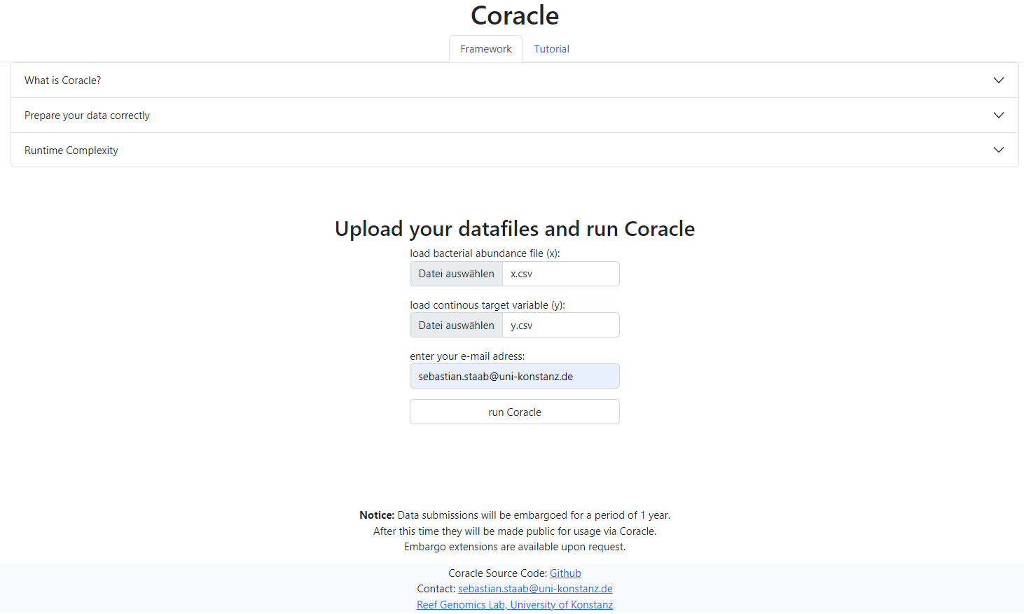
Coracle might take a few minutes to run. If you choose to leave the tab open a landing page will be loaded once Coracle is finished. There you can have a first look at your results, receive a short explanation and a button to download your files as a .csv-file. Additionally, the explanation and a download link for your results will be sent to you to the email-address provided. No registration is necessary. timeout errors can occur while waiting for the result page to load.
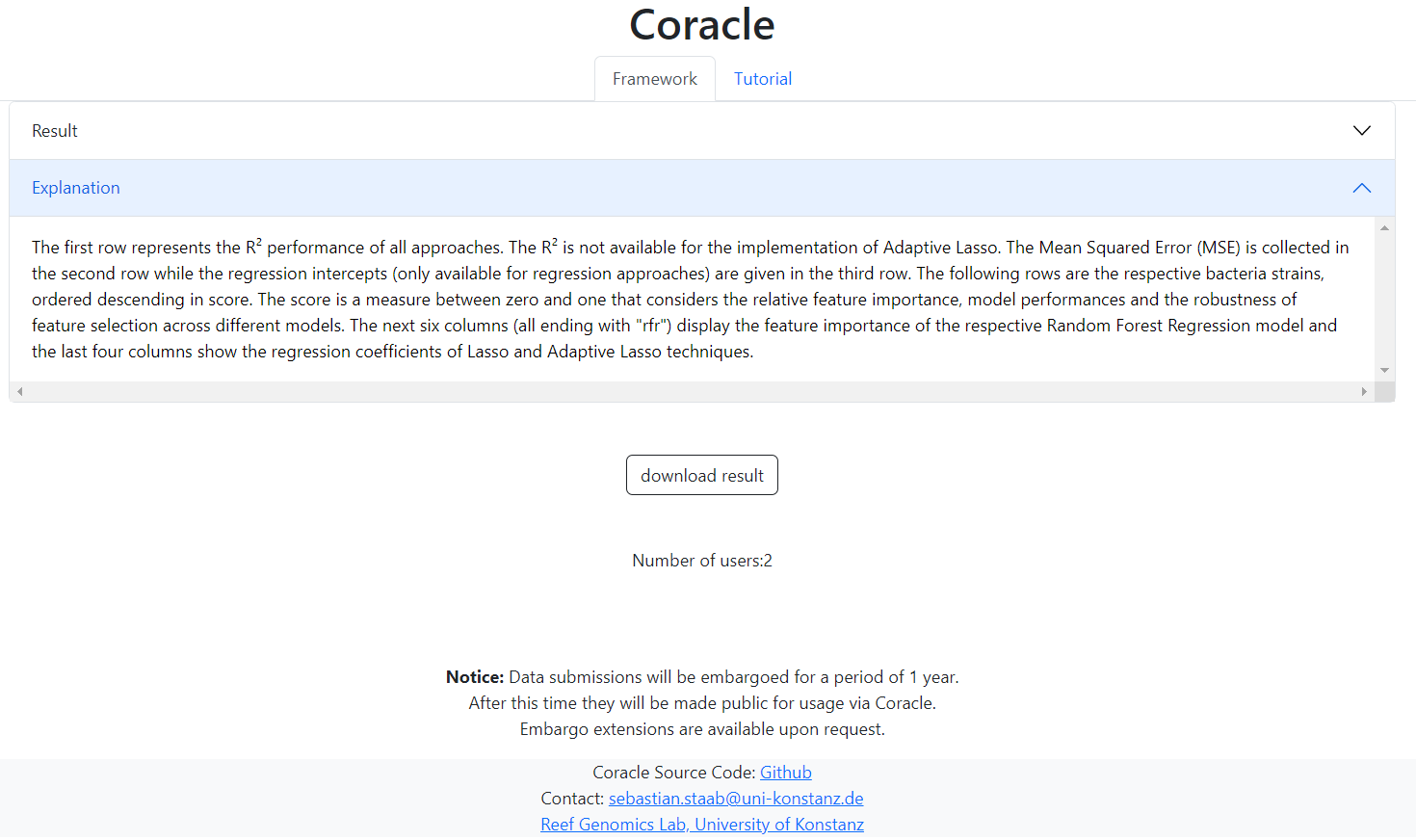
The results can also be found here: